
This document contains supplementary materials for the paper:
Ranking the scores of algorithms with
confidence.
Foucart A., Elskens A., Decaestecker C.
Accepted to ESANN 2025 - Preprint
The file replicate_results.py
contains code to replicate the results presented in the paper. It
requires our cirank
library.
We present in this section details on the statistical tests and confidence interval procedures.
For the bootstrapping method, we proceed as follows: for \(\nu\) repetitions, re-sample \(n\) test cases from the dataset (with replacement) to obtain \(\nu\) bootstrapped samples of the same size as the original test set. In each of these samples \(k \in [1, \nu]\), get the corresponding set of scores \(S^{(k)}_{ij}\), and compute ranks \(r^{(k)}_i\) on the mean score per-algorithm \(S^{(k)}_{i.} = \frac{1}{n}\sum_{j=1}^{n}S^{(k)}_{ij}\), such that \(r^{(k)}_i = 1\) for the lowest value of \(S^{(k)}_{i.}\). Finally, the \(\alpha\)-level confidence interval for algorithm \(i\) is given by the \(\frac{\alpha}{2}\) and \(1-\frac{\alpha}{2}\) percentiles of the distribution of \(r^{(k)}_i\).
First, a Iman-Davenport test1 is performed on all
algorithms, with the null hypothesis \(H_0\) being that the distributions of
scores for each algorithm is the same. To perform this test, the
algorithms are first ranked per-case, so that \(r_{ij} \in [1, m]\) and \(r_{ij} = 1\) means that algorithm \(i\) has the lowest score for test case
\(j\). Then, the average ranks
per-algorithm \(r_{i.} =
\frac{1}{n}\sum_{j=1}^nr_{ij}\) are computed. The test statistic
is \(F_F = \frac{(n-1)Q}{n(m-1)-Q}\),
where \(Q\) is the statistic of the
Friedman test: \(Q =
\frac{12n}{m(m+1)}(\sum_{i=1}^m(r_{i.}^2)-\frac{m(m+1)^2}{4})\).
Under \(H_0\), \(F_F \sim F_{m-1,(m-1)(n-1)}\) where \(F_{a,b}\) is the Fisher-Snedecor
distribution with \(a,b\) degrees of
freedom. scipy.stats.f
is used to compute the critical values of the F-distribution.
If this hypothesis cannot be rejected (p-value \(\geq \alpha\)), then all algorithms have the same confidence interval for their rankings: \([1, m]\). Note that this is different from saying that all algorithms are tied. That would imply that the result of the test proves that the samples are equal, when it merely shows that we cannot reject the hypothesis that they are. The \([1, m]\) confidence interval is therefore a better presentation of the results than, for instance, putting all algorithms tied as first. It correctly shows that the true rank of the algorithms – if they were computed on the population – cannot be resolved based on the available data.
If the null hypothesis is rejected (p-value \(< \alpha\)), then we perform the Nemenyi
post-hoc2 to obtain pairwise comparisons. The
Nemenyi test comparing algorithms \(i\)
and \(i'\) uses the test statistic:
\(Y =
\frac{\sqrt{2}|r_{i.}-r_{i'.}|}{\sqrt{\frac{m(m+1)}{6n}}}\),
which if the two distributions are the same (i.e. under \(H_0\)) should \(\sim q_{m, \inf}\) with \(q_{k, d}\) the Studentized range
distribution for \(k\) groups and \(d\) degrees of freedom. Pairs where \(P(q \geq Y) < \alpha\) are marked as
significantly different, with the sign of \(r_{i.}-r_{i'.}\) determining which is
better or worse. scipy.stats.studentized_range
is used to get the critical values of the studentized range.
The confidence intervals \([L, U]\) are then computed as in Al Mohamad et al.3: \[L = 1 + \text{number of significantly better algorithms}\] \[U = m - \text{number of significantly worse algorithms}\]
The Iman-Davenport test is first performed as described above. If its
null hypothesis is rejected, then we perform the Wilcoxon signed-rank
test4 on all pairs of algorithms, using
either the two-sided or the two one-sided alternatives. scipy.stats.wilcoxon
is used for the pairwise tests.
For each algorithm \(i\), we use
scipy.stats.wilcoxon to compute the p-values of the one- or
two-sided tests with all other algorithms. The p-values are then
adjusted using Holm’s procedure, following the recommendation of Holm,
20135: the \(m-1\) p-values are ordered from most to
least significant. The first value is multiplied by \(m-1\). If the adjusted p-value is \(> \alpha\), the test and all subsequent
tests are deemed non-significant. If it is \(< \alpha\), the test is deemed
significant, and the next value is multiplied by \(m-2\). We repeat until either we get to the
last test (p-value multiplied by 1), or we find a non-significant test.
For the two-sided tests, we also record the sign of the
difference between the mean scores of \(i\) and each other. A “significantly
better” algorithm is therefore an algorithm such that the average score
is higher (assuming higher is better) and the p-value is significant.
For the one-sided tests, we don’t need to record the sign, as each side
give us either the “significantly better” or “significantly worse”
information. The correction for the one-sided tests are applied
“per-side”: first, we adjust the p-values of the tests to the left, then
of the tests to the right (see last section for an example).
Confidence intervals are then computed as above.
For this version of the ranking, a rank transform6 is first applied to the scores \(S_{ij}\), so that \(r_{ij}\) is the global rank of \(S_{ij}\) (i.e. \(r_{ij} = 1\) if \(S_{ij}\) is the lowest score across all algorithms and all test cases). A one-way repeated measures ANOVA is then performed on the global ranks7. As with the Iman-Davenport tests above, a non-rejection of \(H_0\) for the ANOVA leads to a confidence interval of \([1, m] \forall A_i\).
Tukey’s HSD8 is then used, still on the ranks, for the pairwise comparisons, and the confidence intervals are computed based on the numbers of significantly better/worse algorithms.
Rank transformation is performed using scipy.stats.rankdata.
Repeated-measures ANOVA is reimplemented using scipy.stats.f
for the critical values of the F-distribution. Tukey’s HSD is performed
with scipy.stats.tukey_hsd.
Note: this section (2.1) of the supplementary materials has been added on May 19th, 2025, as I realized that it was missing from the originally published material. The analysis itself had been done in October 2024.
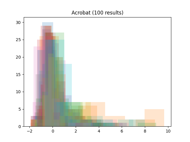
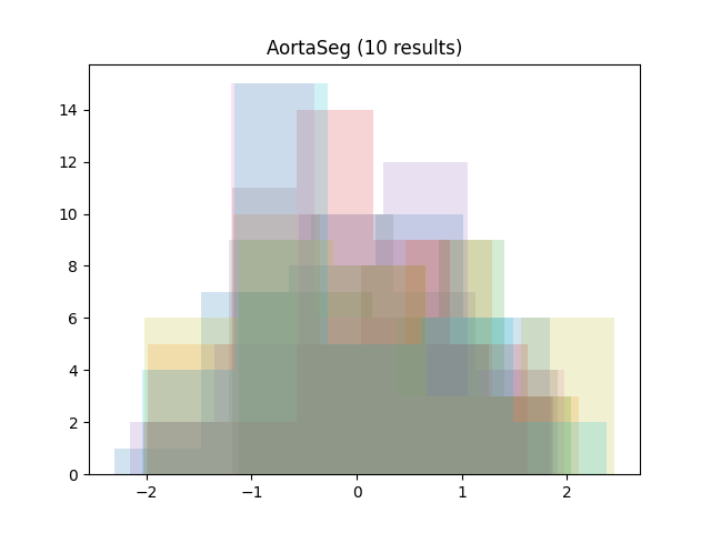
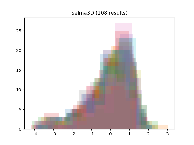
We gathered the results of four recent challenges on grand-challenge.org with per-image numerical evaluation metrics available: the ACROBAT 2024 registration challenge, the AortaSeg 2024 challenge, the CURVAS challenge and the Selma3D. The public leaderboards of each challenge were scraped on October 21nd, 2024, and all available results at that stage were retrieved:
| Challenge | Phase | Number of retrieved results | Number of cases per result |
|---|---|---|---|
| Acrobat | Validation phase | 37 | 100 |
| AortaSeg | Model development phase | 32 | 10 |
| CURVAS | Testing phase | 10 | 65 |
| Selma3D | Preliminary test phase | 50 | 108 |
To focus on the shape of the distributions, all results were standardized by subtracting the mean and dividing by the standard deviation (per team result). Then, all histograms were plotted together (per challenge):
As we can see, the distributions tend to be asymmetrical, with a sharp peak, a long tail and some outliers.
The distribution of the difficulty is a Laplace asymmetric
distribution with \(\kappa=2\), as
implemented in scipy.stats.laplace_asymmetric.
The PDF of that function is shown below:

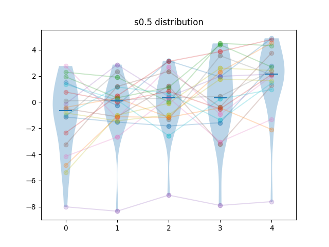
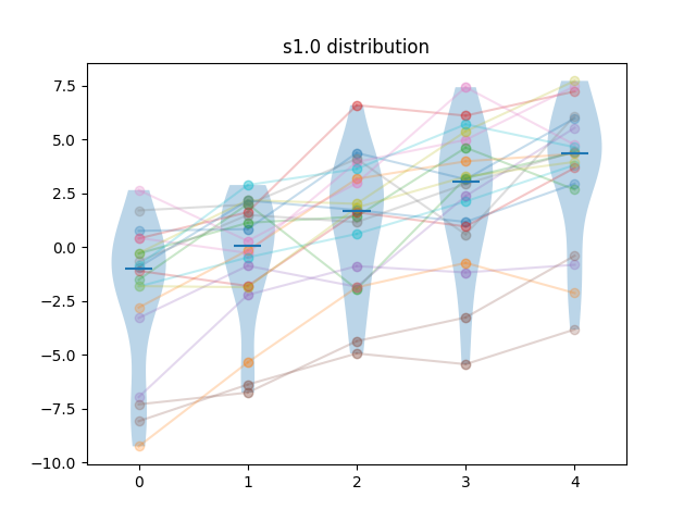
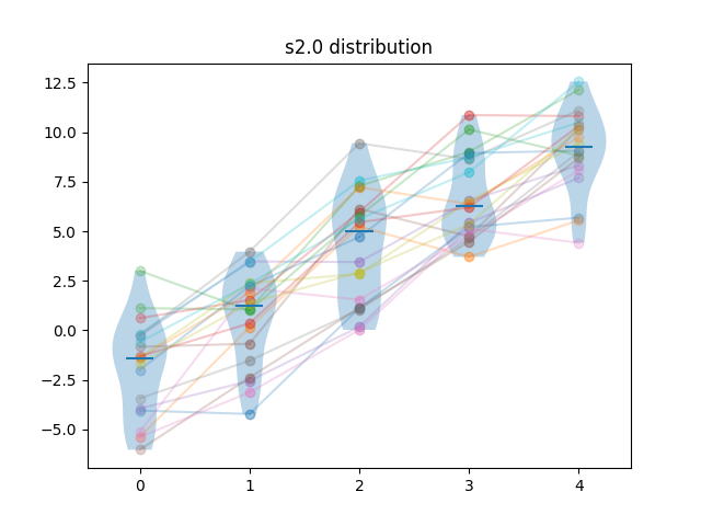
Generated results are obtained by first sampling test cases from the difficulty distribution, then, for each algorithm, adding a sample from a normal distribution. For algorithm \(i\), the mean of that normal distribution is \(i \times f \times \sigma_N\) where \(\sigma_N = \sqrt{\sigma_D}\), and \(\sigma_D\) is the standard deviation of the difficulty distribution, and \(f\) is a separability factor, set at \(0.25, 0.5, 1\) and \(2\) for the different experiments.
So for instance, at separability factor \(0.5\) we would have the scores \(s_{ij} = d_{j} + n_{ij}\), with \(d_{j} \sim L_{\kappa=2}\), \(n_{ij} \sim N(\frac{i\sqrt{\sigma_D}}{2}, \sqrt{\sigma_D})\).
Example of samples of generated results at different separability levels are shown below. Lines show the pairings of the points.

| Method | m=5, n=20 | m=10, n=20 | m=5, n=40 | m=10, n=40 |
|---|---|---|---|---|
| Bootstrap | 33% | 96% | 26% | 94% |
| ID-Nemenyi | 4% | 2% | 4% | 3% |
| ID-Wilcoxon-2S | 4% | 4% | 3% | 5% |
| ID-Wilcoxon-1S | 5% | 4% | 4% | 5% |
| ANOVA-Tukey | 0% | 0% | 0% | 0% |
| Method | FWP | IP | DP | FWDP |
|---|---|---|---|---|
| Bootstrap | 94% | 21% | 0% | 0% |
| ID-Nemenyi | 61% | 11% | 0% | 0% |
| ID-Wilcoxon-2S | 66% | 19% | 2% | 0% |
| ID-Wilcoxon-1S | 68% | 25% | 4% | 5% |
| ANOVA-Tukey | 14% | 2% | 0% | 0% |
| Method | FWP | IP | DP | FWDP |
|---|---|---|---|---|
| Bootstrap | 100% | 50% | 2% | 0% |
| ID-Nemenyi | 61% | 11% | 0% | 0% |
| ID-Wilcoxon-2S | 100% | 60% | 13% | 0% |
| ID-Wilcoxon-1S | 100% | 65% | 18% | 0% |
| ANOVA-Tukey | 88% | 23% | 0% | 0% |
| Method | FWP | IP | DP | FWDP |
|---|---|---|---|---|
| Bootstrap | 100% | 79% | 32% | 6% |
| ID-Nemenyi | 100% | 58% | 0% | 0% |
| ID-Wilcoxon-2S | 100% | 93% | 73% | 43% |
| ID-Wilcoxon-1S | 100% | 93% | 71% | 28% |
| ANOVA-Tukey | 100% | 61% | 5% | 0% |
| Method | FWP | IP | DP | FWDP |
|---|---|---|---|---|
| Bootstrap | 100% | 100% | 99% | 97% |
| ID-Nemenyi | 100% | 60% | 0% | 0% |
| ID-Wilcoxon-2S | 100% | 100% | 100% | 100% |
| ID-Wilcoxon-1S | 100% | 100% | 100% | 100% |
| ANOVA-Tukey | 100% | 95% | 82% | 68% |
Showing in parenthesis the difference with \(0.5\sigma_N\) with \(m=5, n=20\).
| Method | FWP | IP | DP | FWDP |
|---|---|---|---|---|
| Bootstrap | 100% | 64% (+14%) | 6 (+4%) | 0% |
| ID-Nemenyi | 100% (+39%) | 58% (+47%) | 3% (+3%) | 0% |
| ID-Wilcoxon-2S | 100% | 80% (+20%) | 36% (+23%) | 2% (+2%) |
| ID-Wilcoxon-1S | 100% | 81% (+16%) | 38% (+20%) | 1% (+1%) |
| ANOVA-Tukey | 100% (+12%) | 41% (+18%) | 1% (+1%) | 0% |
Showing in parenthesis the difference with \(0.5\sigma_N\) with \(m=5, n=20\).
| Method | FWP | IP | DP | FWDP |
|---|---|---|---|---|
| Bootstrap | 100% | 73% (+23%) | 1% (-1%) | 0% |
| ID-Nemenyi | 100% (+39%) | 46% (+35%) | 0% | 0% |
| ID-Wilcoxon-2S | 100% | 78% (+18%) | 8% (-5%) | 0% |
| ID-Wilcoxon-1S | 100% | 79% (+14%) | 9% (-9%) | 0% |
| ANOVA-Tukey | 100% (+12%) | 47% (+24%) | 0% | 0% |
As mentioned above, Nemenyi’s test statistic is \(Y = \frac{\sqrt{2}|r_{i.}-r_{i'.}|}{\sqrt{\frac{m(m+1)}{6n}}} \sim q_{m, \infty}\) under \(H_0\). In the extreme case where all algorithms have a perfectly monotonic relationship between paired scores (i.e. \(S_{ij} < S_{i'j} \forall i < i'\)), then the ranks for each test case will be \([1, 2... m]\), and the average rank per algorithm will also be \([1, 2... m]\). Thus, the value for \(|r_{i.}-r_{i'.}|\) will be |i’-i| (assuming the indices \(i\) are sorted by their average rank). It will be exactly \(1\) for successive pairs of algorithms. We can therefore compute the minimum sample size \(n\) so that \(P(Q \sim q_{m, \infty} \geq Y) \leq \alpha\). Let \(q_{m, \infty, \alpha}\) be the critical value for the studentized range at significance level \(\alpha\). Then we will reject the null hypothesis for two successive algorithms if:
\[\frac{\sqrt{2}1}{\sqrt{\frac{m(m+1)}{6n}}} \geq q_{m, \infty, \alpha}\]
\[\frac{12n}{m(m+1)} \geq q^2_{m, \infty, \alpha}\]
\[n \geq \frac{m(m+1)}{12}q^2_{m, \infty, \alpha}\]
This gives us the minimum value for the sample size in order for Nemenyi to be able to correctly identify the distributions as fully separated (i.e. all p-values are \(< \alpha\)). For \(m=5\), we already have \(n\geq38\). At \(m=10\), it is \(n\geq184\) (see figure below).

Given two algorithms \(A_i\), \(A_j\) such that the \(A_i\) is “better” than \(A_j\) (\(S_{i.} > S_{j.}\)), the two-sided Wilcoxon test will have higher (i.e. less significant) p-values that the one-sided test where \(H_0\) is \(S_{i.} \leq S_{j.}\). In fact, we will always have \(P_{2S} = 2min(P_{1S}^+, P_{1S}^-)\), where \(P_{1S}^+\) and \(P_{1S}^-\) are the p-values for both sides of the one-sided test.
If we compute the pairwise p-values for \(m\) algorithms, and use these to compute CI for ranks without applying Holm’s correction, we will therefore always have more significant differences between algorithms using the one-sided test. We would therefore expect a much higher power and more Type I errors using this method. This, however, isn’t the case in our experiments.
The reason for that is Holm’s correction. Let us look at an example, using 5 algorithms, a sample size of 20 and a separation factor of \(1.0\). We generate the following results:
The “raw” pairwise p-values (without Holm’s correction) in this sample for the two-sided tests are:
| \(P_{2S}\) | \(A_1\) | \(A_2\) | \(A_3\) | \(A_4\) | \(A_5\) | \(\#_{sba}\) | \(\#_{swa}\) |
|---|---|---|---|---|---|---|---|
| \(A_1\) | - | 3e-2 | 1e-5 | 2e-6 | 2e-6 | 0 | 4 |
| \(A_2\) | 3e-2 | - | 8e-3 | 6e-6 | 2e-6 | 1 | 3 |
| \(A_3\) | 1e-5 | 8e-3 | - | 1e-3 | 6e-6 | 2 | 2 |
| \(A_4\) | 2e-6 | 6e-6 | 1e-3 | - | 1e-3 | 3 | 1 |
| \(A_5\) | 2e-6 | 2e-6 | 6e-6 | 1e-3 | - | 4 | 0 |
For the one-sided test, we have two p-values per pair of algorithms: one for the “test to the left”, one for the “test to the right”. The minimum of those two values is always \(\frac{1}{2}\) as the p-value of the two-sided test. The p-value on the other side are all very close to 1:
| \(P_{1S}^+\) | \(A_1\) | \(A_2\) | \(A_3\) | \(A_4\) | \(A_5\) | \(\#_{swa}\) |
|---|---|---|---|---|---|---|
| \(A_1\) | - | 1e-2 | 5e-6 | 1e-6 | 1e-6 | 4 |
| \(A_2\) | 0.99 | - | 4e-3 | 3e-6 | 1e-6 | 3 |
| \(A_3\) | 1.0 | 1.0 | - | 7e-4 | 3e-6 | 2 |
| \(A_4\) | 1.0 | 1.0 | 1.0 | - | 7e-4 | 1 |
| \(A_5\) | 1.0 | 1.0 | 1.0 | 1.0 | - | 0 |
| \(P_{1S}^-\) | \(A_1\) | \(A_2\) | \(A_3\) | \(A_4\) | \(A_5\) | \(\#_{sba}\) |
|---|---|---|---|---|---|---|
| \(A_1\) | - | 0.99 | 1.0 | 1.0 | 1.0 | 0 |
| \(A_2\) | 1e-2 | - | 1.0 | 1.0 | 1.0 | 1 |
| \(A_3\) | 5e-6 | 4e-3 | - | 1.0 | 1.0 | 2 |
| \(A_4\) | 1e-6 | 3e-6 | 7e-4 | - | 1.0 | 3 |
| \(A_5\) | 1e-6 | 1e-6 | 3e-6 | 7e-4 | - | 4 |
In both the one-sided and two-sided version, the CI for the ranks are completely distinct: \([1, 1], [2, 2], [3, 3], [4, 4], [5, 5]\).
Holm’s correction is applied “row-by-row” on these tables. For each row, we start from the lowest p-value and multiply it by \(m-1 = 4\), then the second by \(m-2 = 3\), until we find a p-value \(> 0.05\), in which case we stop and put all subsequent p-values at 1. In the two-sided approach, the lowest p-value will always correspond to the pair of algorithms that are “furthest away” (so for the first two rows, \(A_5\), for the last two, \(A_1\), and in the middle row it will depend on the exact random sample but in this case it’s \(A_5\)). We end up with the following p-values:
| \(P_{2S}\) | \(A_1\) | \(A_2\) | \(A_3\) | \(A_4\) | \(A_5\) | \(\#_{sba}\) | \(\#_{swa}\) |
|---|---|---|---|---|---|---|---|
| \(A_1\) | - | 3e-2 | 2e-5 | 6e-6 | 8e-6 | 0 | 4 |
| \(A_2\) | 3e-2 | - | 2e-2 | 2e-5 | 8e-6 | 1 | 3 |
| \(A_3\) | 3e-5 | 8e-3 | - | 3e-3 | 2e-5 | 2 | 2 |
| \(A_4\) | 6e-6 | 2e-5 | 3e-3 | - | 1e-3 | 3 | 1 |
| \(A_5\) | 8e-6 | 8e-6 | 2e-5 | 1e-3 | - | 4 | 0 |
For the one-sided test, Holm’s correction is applied separately for each table. This measn that the lowest p-value will be for the “furthest” algorithm on the side being tested:
| \(P_{1S}^+\) | \(A_1\) | \(A_2\) | \(A_3\) | \(A_4\) | \(A_5\) | \(\#_{swa}\) |
|---|---|---|---|---|---|---|
| \(A_1\) | - | 1e-2 | 1e-5 | 3e-6 | 4e-6 | 4 |
| \(A_2\) | 0.99 | - | 8e-3 | 9e-6 | 4e-6 | 3 |
| \(A_3\) | 1.0 | 1.0 | - | 2e-3 | 1e-5 | 2 |
| \(A_4\) | 1.0 | 1.0 | 1.0 | - | 3e-3 | 1 |
| \(A_5\) | 1.0 | 1.0 | 1.0 | 1.0 | - | 0 |
| \(P_{1S}^-\) | \(A_1\) | \(A_2\) | \(A_3\) | \(A_4\) | \(A_5\) | \(\#_{sba}\) |
|---|---|---|---|---|---|---|
| \(A_1\) | - | 1.0 | 1.0 | 1.0 | 1.0 | 0 |
| \(A_2\) | 5e-2 | - | 1.0 | 1.0 | 1.0 | 0 |
| \(A_3\) | 2e-5 | 1e-2 | - | 1.0 | 1.0 | 2 |
| \(A_4\) | 4e-6 | 9e-6 | 1e-3 | - | 1.0 | 3 |
| \(A_5\) | 4e-6 | 3e-6 | 6e-6 | 7e-4 | - | 4 |
In this last table, we know have one non-significant comparison between algorithms \(A_1\) and \(A_2\) (bold). The CI using the one-sided test are therefore no longer completely distinct, as we have: \([1, 1], [1, 2], [3, 3], [4, 4], [5, 5]\).
Thus, even though the one-sided tests by themselves are more powerful than their two-sided counterpart, they may lead to less distinctive CI for the rankings after the application of Holm’s correction to the p-values.
Ronald L. Iman and James M. Davenport. Approximations of the critical region of the Friedman statistic. Communications in Statistics - Theory and Methods, 9(6):571–595, January 1980↩︎
Implemented based on: Janez Demšar. Statistical comparisons of classifiers over multiple data sets. The Journal of Machine Learning Research, 7:1–30, 2006.↩︎
Diaa Al Mohamad, Jelle J. Goeman, and Erik W. Van Zwet. Simultaneous confidence intervals for ranks with application to ranking institutions. Biometrics, 78(1):238–247, March 2022.↩︎
Frank Wilcoxon. Individual Comparisons by Ranking Methods. Biometrics Bulletin, 1(6):80, December 1945.↩︎
Sture Holm. Confidence intervals for ranks. https://www.diva-portal.org/smash/get/diva2:634016/fulltext01.pdf, 2013.↩︎
W. J. Conover and Ronald L. Iman. Rank Transformations as a Bridge between Parametric and Nonparametric Statistics. The American Statistician, 35(3):124–129, August 1981.↩︎
Donald W. Zimmerman and Bruno D. Zumbo. Relative Power of the Wilcoxon Test, the Friedman Test, and Repeated-Measures ANOVA on Ranks. The Journal of Experimental Education, 62(1):75–86, July 1993.↩︎
John W. Tukey. Comparing Individual Means in the Analysis of Variance. Biometrics, 5(2):99, June 1949.↩︎